VLOOKUP is the most-used lookup function in spreadsheets. Most people memorize the syntax without understanding the logic. Once you see how it actually works, you will never forget it.
VLOOKUP scans down the first column of a range until it finds your value, then moves right by a set number of columns and returns what's there. The syntax is =VLOOKUP(lookup_value, table_array, col_index_num, [range_lookup]). Always use FALSE as the 4th argument for exact matching. The most common error is #N/A — it means VLOOKUP could not find the value in your lookup column.
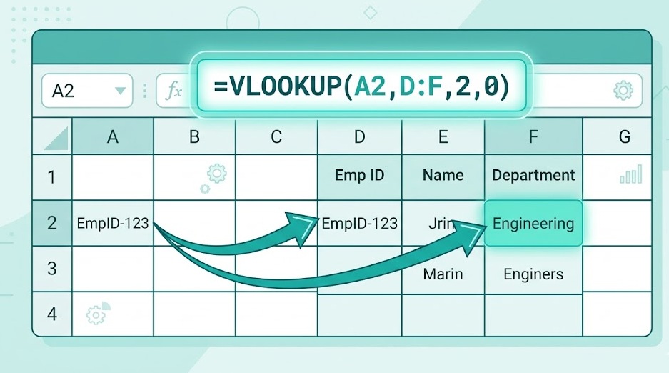
VLOOKUP answers one question: "Find this value in column A — then tell me what's in column C of the same row."
That's it. Everything else is just controlling how it searches and what it returns.
The V stands for vertical. It searches down a column. (HLOOKUP searches across a row — the H stands for horizontal.)
Think of it like a phone book. You scan down the names column (the lookup column) until you find the name you want. Then you move right to find the phone number. VLOOKUP does that automatically — in milliseconds — across thousands of rows.
XLOOKUP is the newer, more powerful alternative. But millions of spreadsheets still use VLOOKUP, many companies run on Excel versions that don't have XLOOKUP, and understanding VLOOKUP makes XLOOKUP trivial to learn. Start here.
| Argument | What It Means | Example |
|---|---|---|
| lookup_value | The value you are searching for. Can be a cell reference, a number, or text in quotes. | A2 or "Smith" |
| table_array | The range containing your data. The first column of this range is always the search column. | B2:E100 |
| col_index_num | Which column of your range to return. 1 = first column (the search column), 2 = second column, and so on. | 3 (returns 3rd column) |
| range_lookup | FALSE = exact match only. TRUE = approximate match (requires sorted data). Default is TRUE — almost always use FALSE. | FALSE |
The default for range_lookup is TRUE (approximate match). If you forget to add the 4th argument, VLOOKUP uses approximate match — and silently returns wrong results without any error. Always type FALSE explicitly.
Imagine this product table starting at cell A1:
| A — Product ID | B — Product Name | C — Price | D — Stock |
|---|---|---|---|
| 1001 | Wireless Mouse | $29.99 | 142 |
| 1002 | USB Hub | $19.99 | 87 |
| 1003 | Monitor Stand | $49.99 | 34 |
| 1004 | Keyboard | $79.99 | 56 |
You want to look up the price of Product ID 1003. Here's the formula:
What VLOOKUP does:
A1:D4) looking for 1003When copying a VLOOKUP formula down a column, lock the table_array with dollar signs so it doesn't shift: =VLOOKUP(A2, $B$1:$E$100, 3, FALSE). Without the lock, Excel adjusts the range as you copy and returns wrong results.
| Exact Match (FALSE) | Approximate Match (TRUE) | |
|---|---|---|
| What it does | Returns result only if a perfect match is found | Returns largest value ≤ lookup value |
| Data must be sorted? | No | Yes — first column must be ascending |
| Wrong results if unsorted? | No (returns #N/A) | Yes — silently returns wrong answer |
| Use for | Almost everything: names, IDs, codes | Numeric ranges: tax brackets, grades, tiers |
| Recommended? | ✅ Always default to this | Only for specific range lookups |
One valid use: commission tiers. If sales of $0–$10,000 = 5% commission, $10,001–$25,000 = 8%, $25,001+ = 12%:
The range E2:E4 must contain 0, 10001, 25001 in ascending order. VLOOKUP finds the largest threshold that doesn't exceed the sales figure and returns the corresponding rate.
Value not found in the lookup column. Check for extra spaces (TRIM), mismatched data types (number vs text), or a genuine missing value. Wrap with IFERROR to suppress.
The col_index_num is larger than the number of columns in your table_array. If your range is 3 columns wide and you asked for column 5, you get #REF!. Count your columns and adjust.
col_index_num is less than 1, or a non-numeric value was used where a number is required. Check your 3rd argument.
Almost always means you forgot FALSE as the 4th argument and got approximate match behavior on unsorted data. Add FALSE and re-check.
=IFERROR(VLOOKUP(A2, $B$1:$E$100, 3, FALSE), "Not found") — replace "Not found" with whatever you want displayed when the lookup fails: a dash, a zero, or a blank "".
If you are on Excel 365, Excel 2021, or Google Sheets — yes. XLOOKUP solves every limitation above: it can look left, handles missing values natively, and doesn't break when you insert columns. For new spreadsheets on supported versions, XLOOKUP is the better choice.
Open any spreadsheet with two related tables. Try matching them with VLOOKUP — it takes under 2 minutes once you know the four arguments.
Step-by-Step Excel VLOOKUP Guide →