VLOOKUP only matches on one value. But real data has multiple conditions — find by region AND product, match by name AND date. Here are three methods to make it work.
VLOOKUP cannot natively match on multiple conditions. The three workarounds: (1) Helper column — concatenate your criteria into one key, VLOOKUP against it. (2) CHOOSE array — build a virtual two-column lookup inside the formula. (3) INDEX/MATCH — the most flexible approach for multi-criteria lookups. All three work in Excel and Google Sheets.
VLOOKUP has one lookup value. It scans one column. It cannot natively check "where Region = East AND Product = Widget AND return the Sales figure."
Imagine this sales table:
| A — Region | B — Product | C — Sales |
|---|---|---|
| East | Widget | $12,400 |
| East | Gadget | $8,900 |
| West | Widget | $15,200 |
| West | Gadget | $6,700 |
You want the sales for East + Widget. A normal VLOOKUP on "East" returns the first East row — which may or may not be Widget. You need AND logic across two columns.
Three solutions follow, from simplest to most powerful.
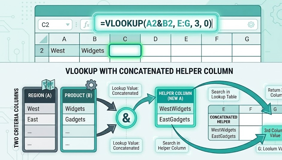
Add a new column (e.g. column D) to your data table that concatenates all the columns you want to match on, separated by a delimiter:
Then VLOOKUP against this combined key using the same delimiter in your lookup value:
Use | or ~ as your separator — not a space or comma, which might appear inside the data values themselves. This prevents false matches where "East W" + "idget" would incorrectly match "East" + "Widget".
The CHOOSE function can create a virtual two-column array — combining two columns into one key on the fly, without touching your source data.
How it works: CHOOSE({1,2}, ...) creates a two-column virtual table where column 1 is the concatenated key and column 2 is the return value. VLOOKUP searches column 1 and returns column 2.
In Excel 2019 and earlier, press Ctrl+Shift+Enter instead of just Enter — this enters it as an array formula (you'll see curly braces around it: {=VLOOKUP(...)}). In Excel 365 and Google Sheets, press Enter normally — dynamic arrays handle it automatically.
INDEX/MATCH can natively handle multiple conditions using array logic. This is cleaner than the CHOOSE workaround and more readable in complex formulas.
How the AND logic works: (A2:A100=F2) returns an array of TRUE/FALSE for each row. Multiplying two such arrays — * — gives 1 only where both conditions are TRUE. MATCH finds the position of the first 1, and INDEX returns the value at that position.
Add more criteria by multiplying another array: *(C2:C100="Q1"). Each additional condition narrows the match further. All conditions must be TRUE for MATCH to find a result.
Sometimes you want to run a VLOOKUP only when certain conditions are met — not multi-criteria matching, but conditional execution.
This formula checks two conditions with AND: Status = "Active" AND Value > 1000. Only if both are true does it run the VLOOKUP. Otherwise it returns "Not eligible". This is different from multi-criteria matching — it is conditional execution of a lookup.
| Situation | Best Method | Why |
|---|---|---|
| You can add a column to your data | Helper column | Simplest, most readable, easiest to audit |
| You cannot modify the source data | CHOOSE array or INDEX/MATCH | Both work without touching the data |
| 3+ conditions | INDEX/MATCH | Most scalable — just multiply more arrays |
| You need to look left | INDEX/MATCH | VLOOKUP can't look left, INDEX/MATCH can |
| Excel 2019 or earlier, avoid array entry | Helper column | No Ctrl+Shift+Enter required |
| Excel 365 or Google Sheets | INDEX/MATCH or XLOOKUP | Dynamic arrays, cleaner syntax |
| Run lookup only under certain conditions | IF + AND + VLOOKUP | Conditional execution, not multi-criteria match |
Multi-criteria lookups are one piece. Understanding how VLOOKUP works end-to-end makes every formula faster to build and easier to debug.
VLOOKUP: Complete Explanation →