VLOOKUP can replace hours of manual data matching with a single formula. This guide walks you through the exact steps — from entering your first VLOOKUP to handling errors and copying it across hundreds of rows.
How to VLOOKUP in Excel: Click an empty cell, type =VLOOKUP(, then enter four arguments: the value to find, the data range (search column must be first), the column number to return, and FALSE for exact match. Example: =VLOOKUP(A2, $D$2:$F$50, 2, FALSE) finds the value from A2 in column D, then returns the value from the 2nd column of the range (column E).
VLOOKUP has one non-negotiable requirement: the column you are searching must be the leftmost column of your table_array.
If you want to look up a customer name by their ID, the ID column must come first. If your data has the ID in column C and name in column A, you either need to rearrange the columns or use INDEX/MATCH instead.
| Works with VLOOKUP ✅ | Does NOT work with VLOOKUP ❌ |
|---|---|
| ID | Name | Email | Phone | Name | ID | Email | Phone (ID is not leftmost) |
| Product Code | Description | Price | Description | Price | Product Code |
Add a helper column: copy or reference the ID column to the far left of your table. Alternatively, use INDEX/MATCH — it has no left-column restriction and is more flexible in every case.
This is the output cell — the cell that will display the value VLOOKUP finds. Usually a blank cell next to the data you want to enrich.
Excel shows the function tooltip listing the arguments. This is your guide as you build the formula.
Click the cell containing the value you want to search for (e.g. A2), or type the value directly in quotes (e.g. "Smith"). Then type a comma.
Click and drag to select the data range. The first column of this range must be the column you're searching. Type a comma when done.
Count from the left of your selected range. Column 1 is the search column itself. Column 2 is one to the right, and so on. Type the number, then a comma.
Type FALSE) for exact match. Press Enter. Your result appears.
This finds the value in A2 by scanning column D, then returns the value from the 3rd column of the range D:G — which is column F.
When you copy a formula down, Excel adjusts cell references automatically. That is usually what you want — but not for the table_array. The search range must stay fixed.
Add dollar signs to lock the table_array:
To add dollar signs quickly: select D2:G100 in the formula bar and press F4. Excel adds the dollar signs automatically.
To copy the formula down: click the cell with the formula, hover over the bottom-right corner until you see a black cross (+), then double-click or drag down.
Reference another sheet in the table_array by prefixing the range with the sheet name followed by an exclamation mark:
If the sheet name contains spaces, wrap it in single quotes:
While typing the formula, when you reach the table_array argument, click the other sheet tab and select the range there. Excel writes the sheet reference automatically — no manual typing needed.
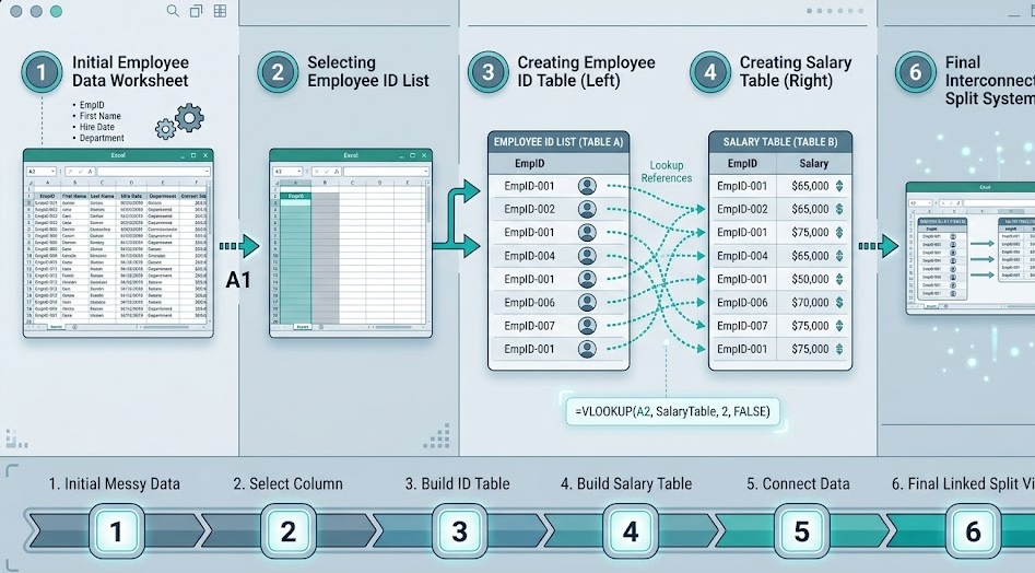
Look up a salary table using employee ID and return the corresponding name or department.
=VLOOKUP(B2, $EmpTable, 2, FALSE)Have a sales order with product codes? Pull the unit price from a separate price table automatically.
=VLOOKUP(A2, PriceList!$A:$C, 3, FALSE)Convert numeric scores to letter grades using approximate match on a sorted grade-boundary table.
=VLOOKUP(C2, $GradeTable, 2, TRUE)Find which items from List A appear in List B. Returns the matched value or #N/A for no match.
=VLOOKUP(A2, $B$2:$B$100, 1, FALSE)Add a country name, account manager, or category to a flat data export using a reference table.
=VLOOKUP(D2, RefTable!$A:$D, 3, FALSE)Apply tiered tax rates to income figures using approximate match on a sorted rate table.
=VLOOKUP(B2, $TaxTable, 2, TRUE)| Error / Symptom | Cause | Fix |
|---|---|---|
| #N/A | Value not found in lookup column | Check for spaces (use TRIM), mismatched types, or wrap in IFERROR |
| #REF! | col_index_num exceeds range width | Count your columns; reduce col_index_num or widen the range |
| #VALUE! | col_index_num is < 1 or non-numeric | Ensure 3rd argument is a whole number ≥ 1 |
| Wrong value, no error | Missing FALSE — using approximate match | Add FALSE as 4th argument |
| Formula shifts when copied | Table range not locked | Add $ to table_array: press F4 on the range |
| #N/A on numbers | Numbers stored as text (or vice versa) | Use VALUE() to convert: VLOOKUP(VALUE(A2),...) |
=IFERROR(VLOOKUP(A2, $D$2:$F$100, 2, FALSE), "") — surround any VLOOKUP with IFERROR to return a blank, dash, or custom message instead of an error code. Clean reports, no red cells.
The most powerful use of VLOOKUP is matching and comparing data across two lists. See exactly how to do it.
VLOOKUP: Compare Two Columns →