VLOOKUP in Google Sheets works identically to Excel — same syntax, same logic. But Sheets has a few quirks worth knowing, plus full XLOOKUP support that makes some tasks much simpler.
VLOOKUP in Google Sheets: =VLOOKUP(search_key, range, index, [is_sorted]). Use FALSE for exact match. Example: =VLOOKUP(A2, D2:F100, 2, FALSE) finds A2's value in column D, returns the value from column E. Cross-tab lookups use single quotes around the sheet name: =VLOOKUP(A2, 'Sheet2'!A:C, 2, FALSE). Google Sheets also supports XLOOKUP natively — consider it for new formulas.
| Argument | What It Does | Tip |
|---|---|---|
| search_key | The value to find (cell reference or literal) | Use a cell reference so the formula works for multiple rows |
| range | The data range; first column is the search column | Lock with $ signs when copying down: $A$2:$C$100 |
| index | Column number to return (1 = first col of range) | Count from the left edge of your range, not the sheet |
| is_sorted | FALSE = exact match; TRUE = approximate (sorted data) | Always use FALSE unless doing numeric range lookups |
Google Sheets uses slightly different argument names than Excel (search_key vs lookup_value, is_sorted vs range_lookup) — but the behavior is identical.
You have an order list in columns A–B and a product price table in columns D–F:
| A — Order ID | B — Product Code | D — Product Code | E — Name | F — Price | |
|---|---|---|---|---|---|
| ORD-001 | P-103 | P-101 | Notebook | $4.99 | |
| ORD-002 | P-101 | P-102 | Pen Set | $8.99 | |
| ORD-003 | P-105 | P-103 | Highlighter | $3.49 |
To pull the price for each order into column C:
VLOOKUP finds P-103 in column D, moves to the 3rd column of the range (column F), and returns $3.49. Copy down to C3 and C4 for the other orders.
In Google Sheets, you can use entire column references like D:F instead of $D$2:$F$1000. This handles any number of rows automatically: =VLOOKUP(B2, D:F, 3, FALSE). Avoid this in Excel with large datasets — it slows recalculation. In Sheets it's generally fine.
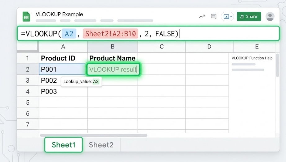
Reference another sheet by its tab name followed by an exclamation mark. Always wrap the tab name in single quotes in Google Sheets:
While typing your formula and you reach the range argument, click the other tab and select the range there. Google Sheets writes the sheet reference automatically — including the single quotes and exclamation mark.
VLOOKUP cannot directly reference another Google Sheets file. Use IMPORTRANGE to bring the data in first, then VLOOKUP against it:
Google Sheets VLOOKUP supports wildcard characters when using exact match (FALSE):
| Wildcard | Meaning | Example | Matches |
|---|---|---|---|
* | Any number of characters | "Jo*" | John, Johnson, Joseph |
? | Any single character | "J?n" | Jan, Jon, Jun |
~* | Literal asterisk | "10~*" | Finds "10*" exactly |
If multiple rows match your wildcard pattern, VLOOKUP returns only the first one it finds. For multiple matches, use FILTER: =FILTER(B2:B100, REGEXMATCH(A2:A100, "^Pro")).
| Error | Cause | Fix |
|---|---|---|
| #N/A | Value not found in search column | Check for spaces (TRIM), type mismatches, use IFERROR |
| #REF! | Index number exceeds range width | Reduce index or expand your range |
| #ERROR! | Formula syntax issue | Check commas, brackets, and quote marks |
| Wrong result | is_sorted omitted (defaults to TRUE) | Add FALSE as the 4th argument explicitly |
| #N/A on numbers | Number stored as text | Wrap lookup value: VALUE(A2) or TEXT(A2,"0") |
XLOOKUP is available in all Google Sheets accounts. It solves VLOOKUP's biggest limitations:
| Task | VLOOKUP | XLOOKUP |
|---|---|---|
| Look up value to the left of search column | ❌ Not possible | ✅ Works natively |
| Handle missing values cleanly | Needs IFERROR wrapper | Built-in if_not_found argument |
| Insert column without breaking formula | ❌ Breaks | ✅ Range-based, not index-based |
| Return multiple columns at once | ❌ One formula per column | ✅ Returns an array |
| Existing spreadsheets and Excel compatibility | ✅ Universal | Sheets: yes; older Excel: no |
Cleaner: you specify the search column and return column separately, so inserting columns never breaks it.
One of the most useful VLOOKUP patterns in Google Sheets is matching two lists to find what's in one but not the other.
VLOOKUP: Compare Two Columns →