Two lists. You need to know what's in both, what's only in one, and what's missing. VLOOKUP does this in seconds — once you know the right formula for each scenario.
To compare two columns with VLOOKUP, use one column as the lookup value and the other as the search range. =IF(ISNA(VLOOKUP(A2, $C$2:$C$100, 1, FALSE)), "Missing", "Match") checks each value in column A against column C and labels it. Returns "Match" if found, "Missing" if not. Works in Excel and Google Sheets.
When comparing two columns, you are not returning data from a separate table. You are checking whether a value exists in another column.
The trick: set the col_index_num to 1. This makes VLOOKUP return the matched value itself (column 1 of the range) — which you can then use with ISNA or IFERROR to determine whether the match was found.
You then wrap this with IF + ISNA (or IFERROR) to turn the #N/A into a readable label.
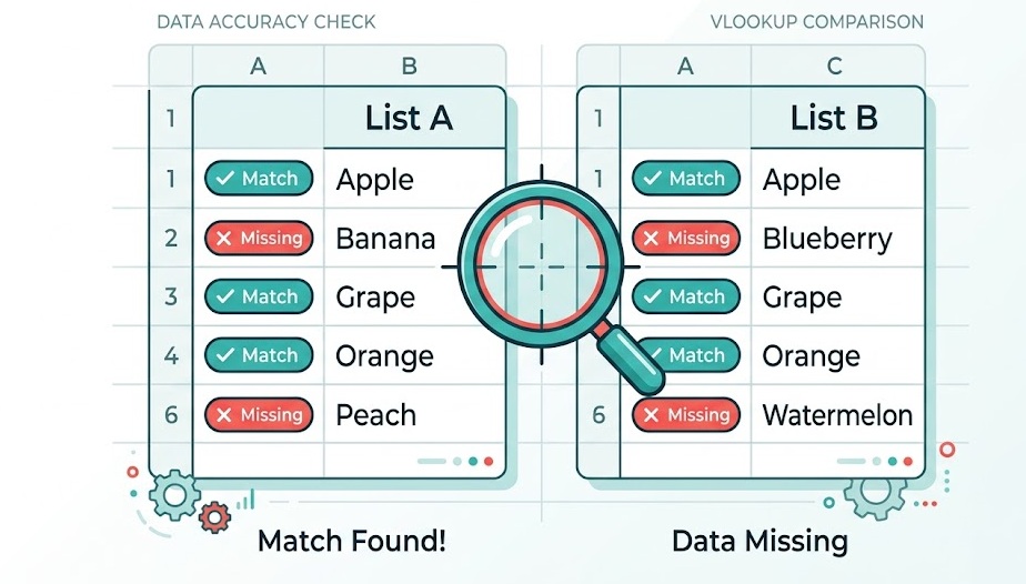
You have List A in column A and List B in column C. You want to know which values from List A appear in List B.
Result: column B shows the matched value where A2 exists in column C — blank where it doesn't. Filter column B to non-blank values to see only matches.
| A — List A | B — Formula Result | C — List B |
|---|---|---|
| Apple | Apple | Banana |
| Mango | Apple | |
| Banana | Banana | Grape |
| Cherry | Peach |
You want to know what's in column A that does NOT appear in column C. These are your gaps.
Filter column B for "Missing" to see only the values from List A that don't appear in List B.
After flagging with the formula above, use Filter → Filter by value → "Missing" to see only the gaps. In Excel 365 or Google Sheets, use the FILTER function to extract them directly: =FILTER(A2:A100, ISNA(VLOOKUP(A2:A100, $C$2:$C$100, 1, FALSE)))
The cleanest version: every row in column B gets a clear label — no blanks, no #N/A errors.
Copy this formula down column B for every row in List A. Sort column B to group matches and non-matches together instantly.
Sometimes you don't just want to confirm a match — you want to pull a related value from the matched row. This is classic VLOOKUP territory.
List A is in column A (customer IDs). Column C has customer IDs, column D has their status. You want to pull the status into column B for each ID in List A:
Note the table_array is now $C$2:$D$100 (two columns) and col_index_num is 2 — returning column D (the status column).
Clean boolean label for each row in List A.
=IF(ISNA(VLOOKUP(A2,$C:$C,1,FALSE)),"No","Yes")Useful for filtering — blank rows are non-matches.
=IFERROR(VLOOKUP(A2,$C:$C,1,FALSE),"")Dynamic array — spills all missing items at once.
=FILTER(A2:A100,ISNA(VLOOKUP(A2:A100,$C:$C,1,FALSE)))Single number — how many matches exist.
=COUNTIF($C:$C,A2) — then SUM the columnMatch and pull related data in one formula.
=IFERROR(VLOOKUP(A2,$C:$D,2,FALSE),"—")Compare List A on Sheet1 against List B on Sheet2.
=IF(ISNA(VLOOKUP(A2,Sheet2!$A:$A,1,FALSE)),"Missing","Match")For a pure match/no-match check, COUNTIF is simpler and faster than VLOOKUP:
| Use Case | Best Formula | Why |
|---|---|---|
| Does value exist in other column? | COUNTIF | Simpler, no #N/A handling needed |
| Return data from matched row | VLOOKUP | COUNTIF can't return related data |
| Count how many matches exist | COUNTIF | Direct count, one formula |
| Compare values in same row (A2 vs B2) | IF(A2=B2,...) | Direct equality — no lookup needed |
| Extract all non-matching rows | FILTER + ISNA | Dynamic, updates automatically |
Combining VLOOKUP with AND lets you match on multiple criteria at once — a common need in real data work.
VLOOKUP + AND Function →